Task #208
closed
Prepare and process Indian Ocean Tuna Commission catch statistics
100%
Description
In order to support and promote processing of stock assessment data in BlueBridge, we were requested to analyse tuna catch statistics and demonstrate the capabilities of the e-Infrastructure.
This ticket will report the preparation and processing activity required to extract indicators and trends from data published by the Indian Ocean Tuna Commission (an IRD stakeholder), and to demonstrate the D4Science capabilities in this domain.
Files
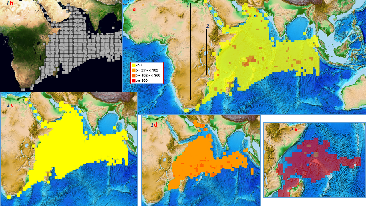
| Figure1.png (2.31 MB) Figure1.png | Distribution of fishing effort locations with enlargements focusing on different ranges of fishing rate | ||
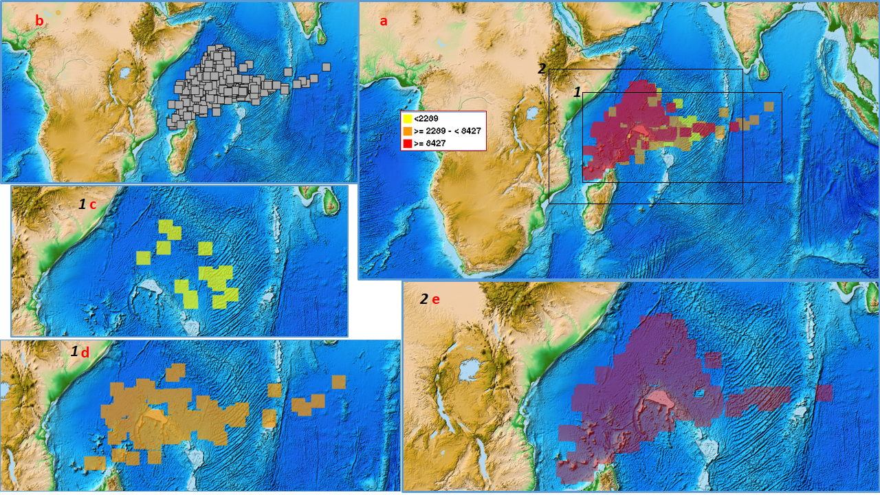
| Figure2.png (2.65 MB) Figure2.png | Distribution of barycenters fishing effort locations with enlargements focusing on different ranges of fishing rate | ||
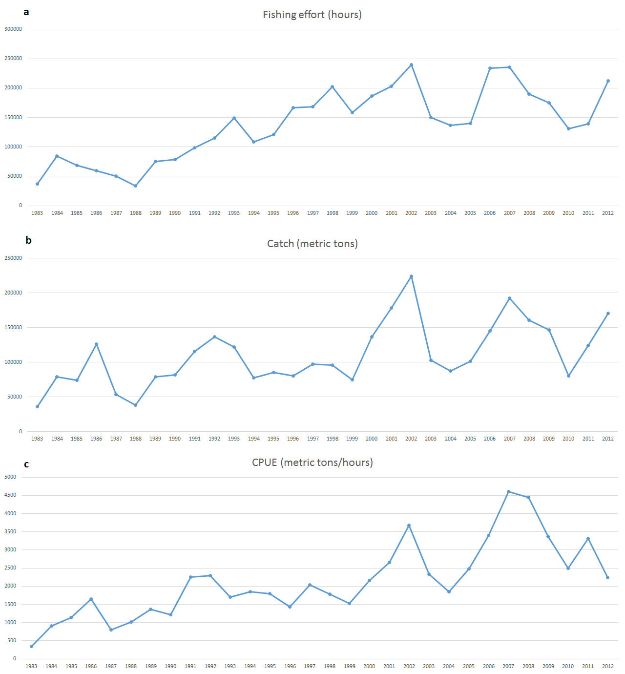
| Figure4.png (58.9 KB) Figure4.png | Annual trends of fishing hours, catch and CPUE | ||
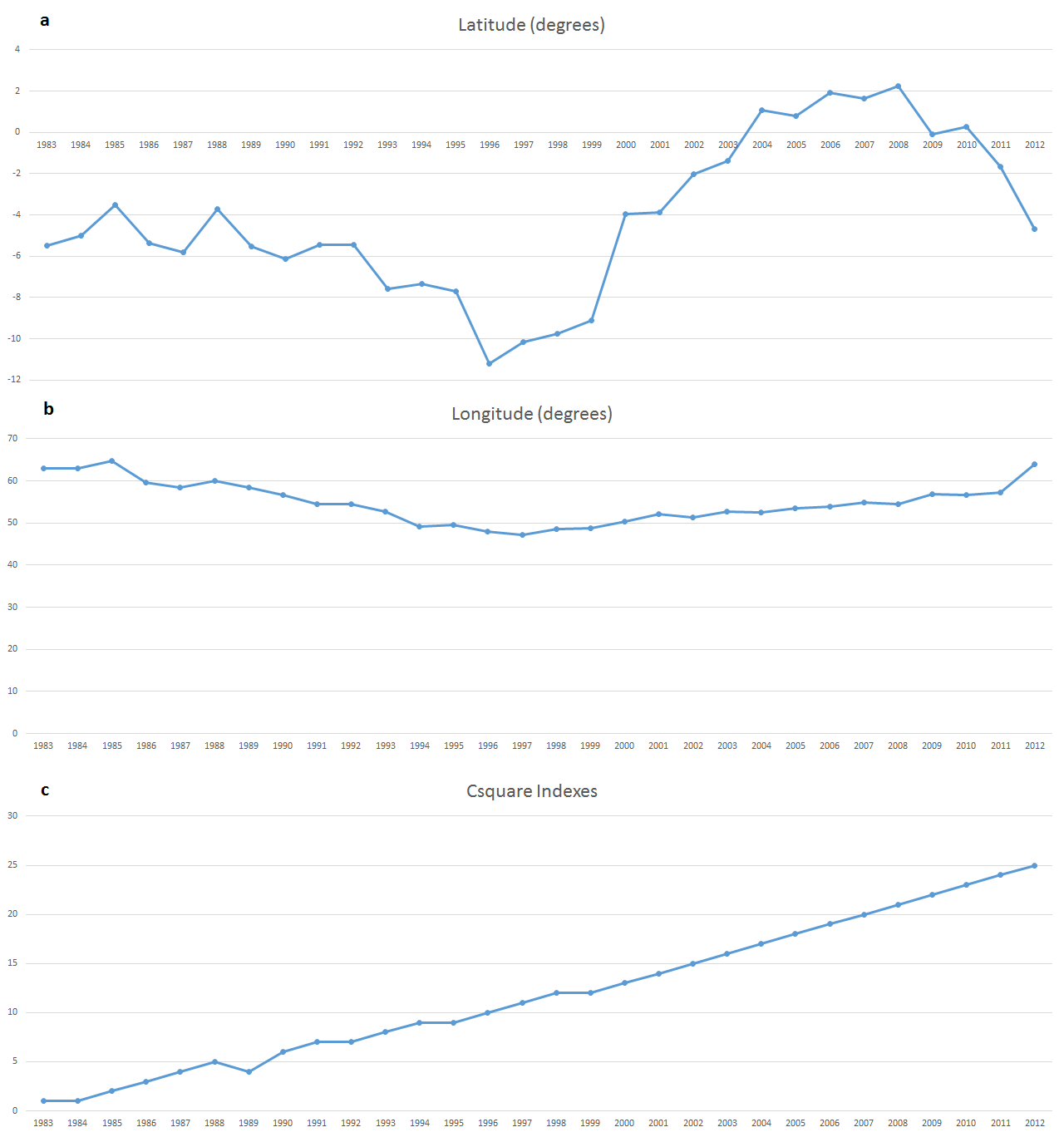
| Figure6.png (44.9 KB) Figure6.png | Annual trends of longitude, latitude and csquare indexes | ||
| Figure3.png (194 KB) Figure3.png | Monthly trends of fishing effort, catch and CPUE | ||
| Figure5.png (175 KB) Figure5.png | Monthly trends of latitude, longitude and csquare indexes | ||
| Figure7.png (597 KB) Figure7.png | |||
| Figure8.png (38.9 KB) Figure8.png | |||
| Figure9.png (50.9 KB) Figure9.png | |||
| Table 1.xlsx (14.2 KB) Table 1.xlsx | Inner periodicities of the trends | ||
| Figure10.png (92.2 KB) Figure10.png | Example of spectrogram of the fishing effort with analysis window length of 128 samples | ||
| Figure11.png (244 KB) Figure11.png | |||
| Figure12.png (118 KB) Figure12.png | |||
| Figure13.png (770 KB) Figure13.png | |||
| Table 2a.xlsx (9.72 KB) Table 2a.xlsx | |||
| Table 2b.xlsx (9.04 KB) Table 2b.xlsx | |||
| Table 3.xlsx (9.7 KB) Table 3.xlsx | |||
| ForecastingTimeSeriesAbstract 2.0.docx (14.3 KB) ForecastingTimeSeriesAbstract 2.0.docx |
 Updated by Gianpaolo Coro about 11 years ago
In this ticket we report a process for catch statistics having the following aims:
- producing the trends of the most exploited locations
- producing aggregated statistics of a stock exploitation
- finding periodic patterns in portions of the trends of fishing effort,CPUE and exploited areas
- highlighting if these patterns are found at annual other than monthly time granularity
- predicting future fishing locations, effort, catch and CPUE
- detecting general shifts in time of the most exploited areas
The difficulty here is to find an automatic method producing the information above. Today, signal processing and data mining techniques are used by specialists to extract this information, although few examples are available for fisheries statistics, because these are signals whose statistical properties vary in time (non-stationary signals). Most predictive models use growth equations, life history traits or population dynamics to project a catch trend in the future. On the other hand, often they do not take into account other non-ecological factors that could have modified a catch trend, such as piracy activity, overfishing and law regulations.
Thus, the challenge is to find a completely automatic method that does the job of a signal processing specialist and is applicable to fisheries statistics. The method should require the minimal parametrisation. The method will automatically find periodic patterns and possibly a structure behind pieces of a trend. These will allow reconstructing the signal and to project it in the future.
As benchmark data, we will use the Indian Ocean Tuna Commission reports between 1983 and 2013 for the purse seine fishing of the yellowfin tuna.
Updated by Gianpaolo Coro almost 11 years ago
- % Done changed from 0 to 10
In the following, I report a workflow for this activity. The approach will use catch statistics by IOTC as a case study. In particular, IOTC catch reports for yellowfin tuna with purse seine technique will be used. The dataset is available on the IOTC website (and here http://goo.gl/yVKBLk). The reports include monthly information between 1981 and 2013.
The method follows this workflow:
- Visualise and inspect time series of fishing effort, catch, CPUE, latitude and longitude (the dimensions of the dataset) both geographically and as mono-dimensional signals.
- Since reports overlap in time and space, aggregate information by summing overlapping reports. At this stage, there will be several location associated to one time instant.
- In order to work on one time series for each dimension, produce one representative for all the locations associated to the same time instant: take the barycentre of the fishing locations. The barycentre accounts for the number of fishing hours spent by vessels in each location and will be close to the most exploited locations.
- Produce statistics and trends for the dimensions with monthly and annual temporal granularity.
- Report the most exploited locations in terms of fishing hours, along with their statistical properties.
- Using short-time Fourier analysis on each dimension, discover hidden periodic patterns in the signals and in their portions.
- Discover an approach to model the non-stationary time series (i.e. having statistical properties which vary in time) of the dimensions and to forecast them in the future. This approach should be based on the analysis of a trend and should autonomously discover a structure in the time series.
- Train the model with the time series up to the last year and use the last reporting year (2013) as a reference to evaluate the quality of the forecast.
- Compare the discovered method with other 3 approaches commonly used to forecast time series in fisheries.
- Discuss the discovered properties, the forecasts and the usage of this technique.
Point 7 is necessary because current forecasting approaches have several drawbacks:
a. They reach good performance only when the signal is stationary or contains periodicities
b. They require configuring several parameters and involving a signal processing expert
The Fourier analysis and the forecasting methods presented here will overcome the above issues.
Updated by Gianpaolo Coro almost 11 years ago
- File Figure1.png Figure1.png added
- File Figure2.png Figure2.png added
- File Figure3.png added
- File Figure4.png Figure4.png added
- File Figure5.png added
- File Figure6.png Figure6.png added
- % Done changed from 10 to 20
The attached figures report several representations of the benchmark IOTC data. Figure 1 and 2 show the spatial distribution of the involved fishing locations and of their respective barycenters per month. The colors refer to different amounts of hours.
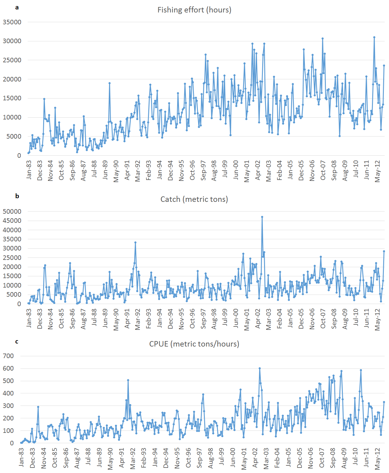
Figure 3 and 4 report the trends of fishing effort, catch and CPUE in the barycenters, per month and per year.
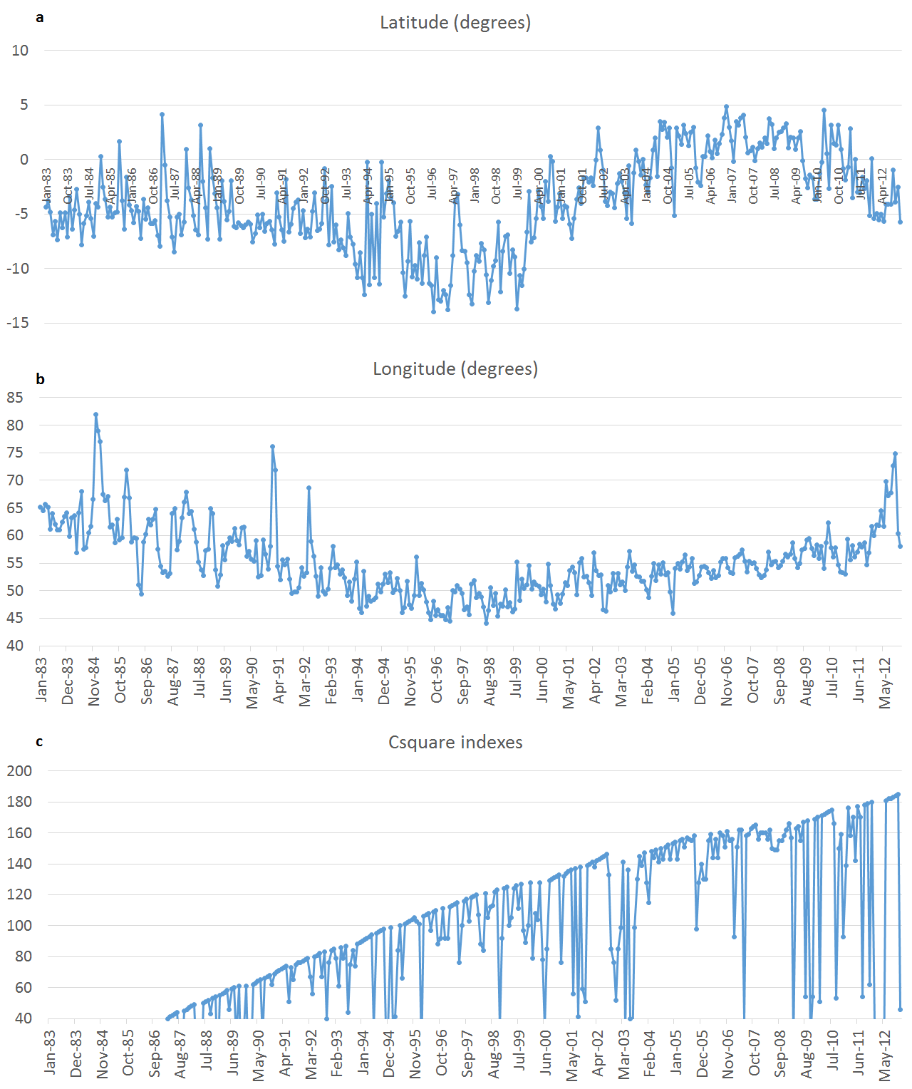
Figure 5 and 6 report the same trends for latitudes, longitudes and barycenters csquares.
The chart for csquares has been built by associating a unique index to the csquares occupied by the monthly barycenters. It shows that during the past 30 years some locations are still exploited, but overall there are always new locations exploited each year. This can be deduced by looking at the increasing linear trend of the csquares distribution.
It is evident that none of the trends is stationary, because variances and means change in time. This is highlighted by the annual trends, which are essentially a smoothed version of the monthly trends.
Periodicity and seasonality should be searched in the monthly trend, at finer temporal granularity.
Updated by Gianpaolo Coro almost 11 years ago
- File Figure3.png Figure3.png added
- File Figure5.png Figure5.png added
Updated by Gianpaolo Coro almost 11 years ago
- File Figure7.png Figure7.png added
- File Figure8.png Figure8.png added
- File Figure9.png Figure9.png added
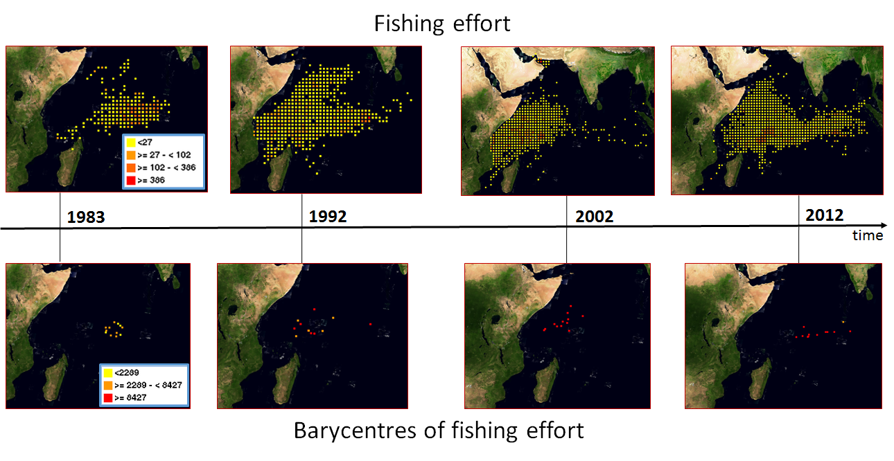
Figure 7 reports the spatial extension of the overall fishing locations and of their respective barycenters at different times.
These charts highlight that the geographical extension of the fishing activity increases in time and also that the effort in the barycenters becomes higher (points become more red). The increasing number of exploited locations in Figure 7 agrees with the indications of the csquare indexes chart.
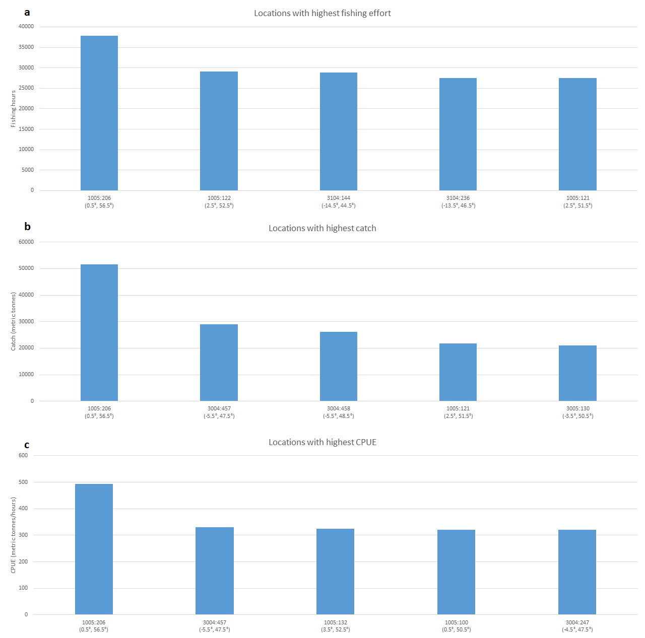
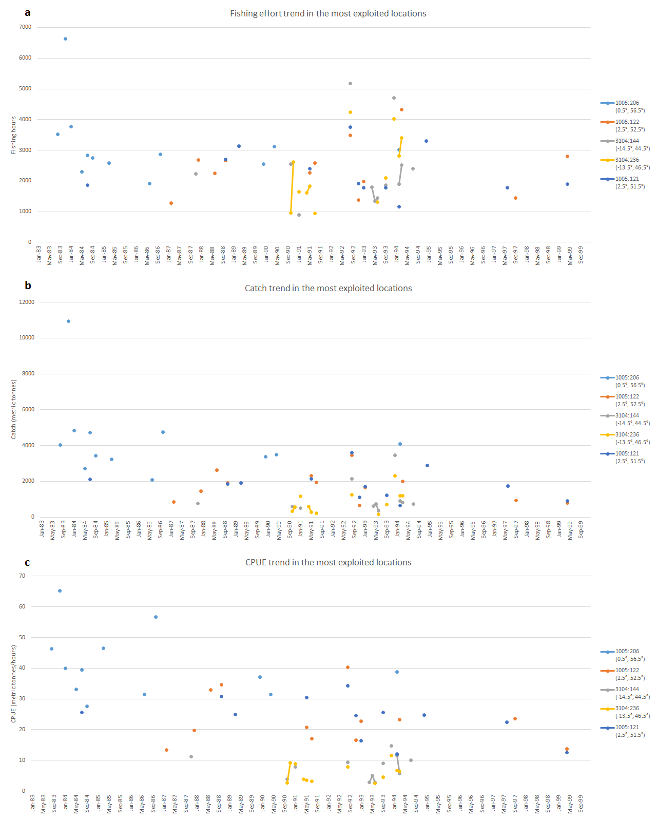
Figure 8 reports the most exploited locations in the 30 years span of the dataset and Figure 9 reports the trends of the fishing effort in these locations. It is notable that all the exploitation trends finish before 2000 and present uniform sampling periods, sometimes concentrated in few years.
This could indicate that these areas have been hardly exploited and their productivity lowered before 2000.
Updated by Gianpaolo Coro almost 11 years ago
- File Table 1.xlsx Table 1.xlsx added
- File Figure10.png Figure10.png added
- % Done changed from 20 to 50
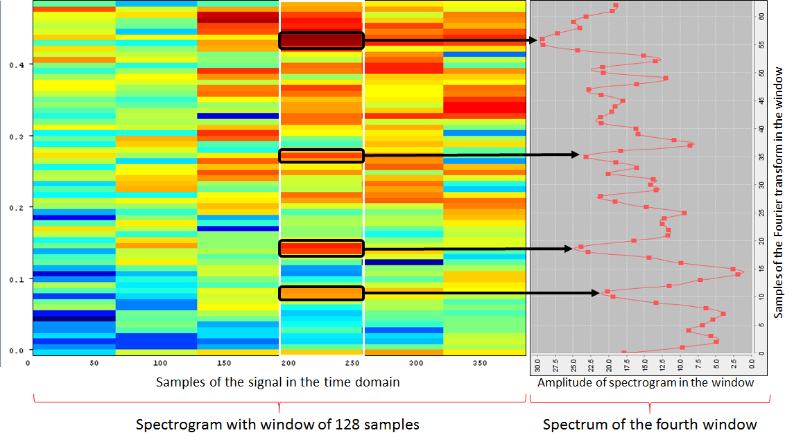
In order to discover inner periodicities in the trends, we applied short-time Fourier analysis. This technique uses a sliding window on the signal and, for each window, it reports the periodic components of the selected portion of signal (Spectrum). The peaks of the Spectrum are the highest periodic components.
We used the standard Fast Fourier Transform (FFT) algorithm to compute the Fourier transform in each window. This algorithm gains maximum performance when the number of window samples is multiple of 2.
The (uniformly sampled) fishing effort signal has length 360, thus we applied the FFT windowed analysis using window lengths ranging from 16 to 256 samples (with a slide of the window equal to half of the window length). In particular, we used the following windows: 16 samples (1 year), 32 samples (2 years and half), 64 samples (4 years and 9 months), 128 samples (9 years and half) and 256 samples (9 years and half).
Figure 10 (the Spectrogram) shows one example of short time FFT analysis applied to the fishing effort trend, where each vertical colored band is the Fourier transform of a portion of a signal. Red bars refer to peaks of frequency strength. The figure shows the Spectrum of the central band, which presents four main periodic components.
The complete analysis is reported in the attached table (Table 1). The different window lengths emphasize different periodic components. Signals presents periodicities of 3 months (3.5 samples), sometimes of 4 months (5 samples), 6 months (7.5 samples), 9 months (10.33 samples) and 11 months (12.6).
Fishing effort, catch and CPUE present also periodic components of 60 months (63.75 samples).
Latitude and longitude present periodicities between 3 and 9 months in several time frames. Random checks on these intervals confirm these properties.
Obviously, the analysis above was automatized on the basis of the signal length, thus is applicable to other signals.
Updated by Gianpaolo Coro almost 11 years ago
- File Figure11.png Figure11.png added
- File Figure12.png Figure12.png added
- File Figure13.png Figure13.png added
- File Table 2a.xlsx Table 2a.xlsx added
- File Table 2b.xlsx Table 2b.xlsx added
- File Table 3.xlsx Table 3.xlsx added
- % Done changed from 50 to 80
As last step, we forecasted the signals of the barycentres for 2013, given the history of data between 1983 and 2012.
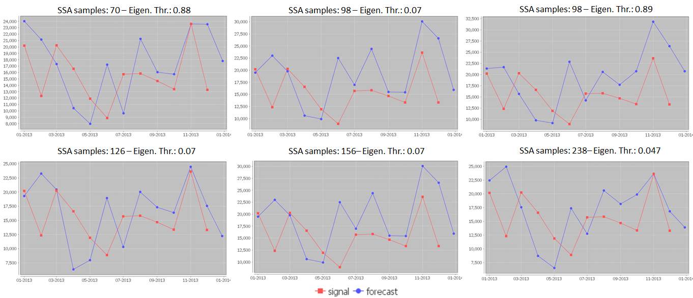
These trends are very complex non-stationary signals, but present inner periodic portions. Thus, we chose a forecasting algorithm that could manage this scenario. One of the most powerful models in these cases is Singular Spectrum Analysis (SSA), which tries to “understand” the inner structure of a signal before reconstructing it. SSA divides the signal in chunks, the chunks are superposed to form a matrix and eigenvalues of the matrix are extracted. These represent the inner structure of the signal and allow reconstructing it in the future.
For this experiment, we used an implementation of SSA called Caterpillar-SSA, which accepts two input parameters: the length of the chunking window (SSA samples) and a threshold for the eigenvalues (to select only the ones with higher values, Eigen. Thr.). The combination of these two parameters produces a large amount of forecasts (see Figure 11 for some examples). We produced forecasts by varying SSA samples and eigenvalues thresholds. In particular, we increased the number of SSA samples of one unit per each experiment. For each fixed number of SSA samples, we used eigenvalues thresholds at 30, 40, 50, 60 percentiles of the eigenvalues list.
In order to filter this set of solutions and choose the best forecast, we applied the following rationale to each signal:
- We first selected only the forecasts having statistical properties (variance, mean, maximum and minimum values) similar to the signal in 2012. We defined the similarity as a relative difference of less than 50% for each statistical property.
- We chose the best forecast as the one having overall most similar statistical properties, i.e. the one having the lowest product of the relative differences. Table 2a reports the relative differences for several forecasts of the fishing effort. It is notable that the one using 126 SSA samples and 0.07 Eigen. Thr. is the best forecast according to our rationale.
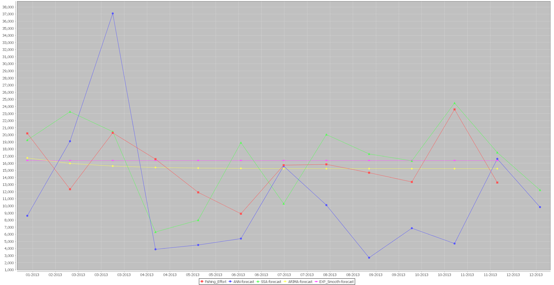
In order to verify the quality of this forecast, we evaluated it similarity with respect to the true signal in 2013. We compared also other commonly used approaches from literature: artificial neural networks, ARIMA and exponential smoothing. Figure 12 reports a comparison between these forecasts, and it is notable that the SSA forecast (green) is the one that best resembles the true signal (red). A numerical comparison is reported in Table 2b, which confirms the overall best similarity by the SSA forecast to the true signal.
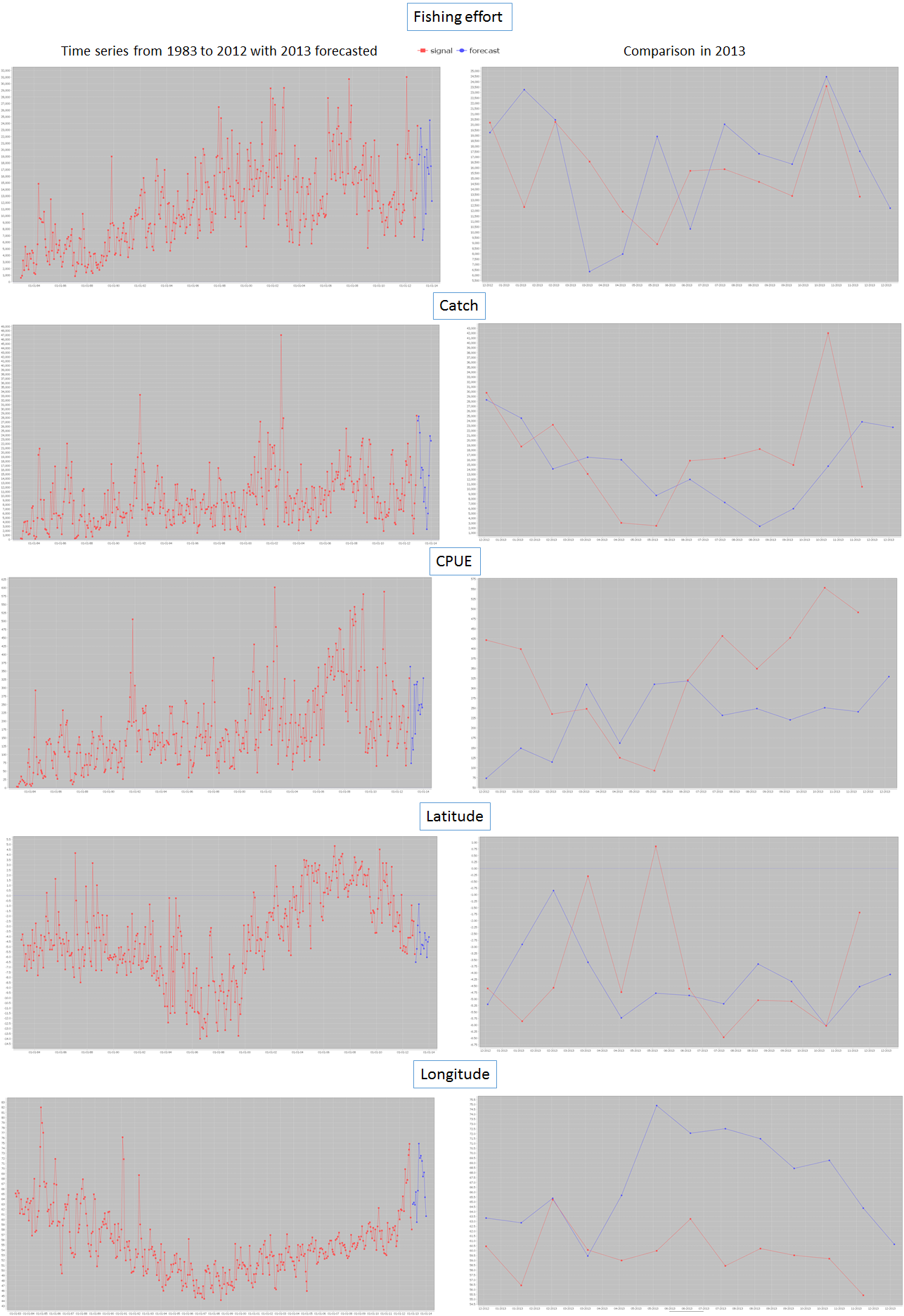
Applying the SSA process above to all the trends of the dimensions (fishing effort, catch, CPUE, latitude and longitude) produces the forecasts in Figure 13.
Table 3 reports the best SSA parameters for each dimension and the similarity with respect to the 2012 and 2013 trends.
Updated by Gianpaolo Coro almost 11 years ago
- % Done changed from 80 to 90
This ticket demonstrates how the D4Science e-Infrastructure is able to operate advanced management and processing of fisheries data. In particular, we used fisheries data (IOTC time series) which will be of interest to the BlueBridge project.
Data management and GIS maps was produced using TabMan, whereas we used StatMan for data processing. Cloud computing allowed running multiple experiments at the same time using different parameters.
In this experiment, we used both web interfaces and service clients (to automatize routine executions).
Updated by Gianpaolo Coro almost 11 years ago
- File ForecastingTimeSeriesAbstract 2.0.docx ForecastingTimeSeriesAbstract 2.0.docx added
- Status changed from In Progress to Closed
- % Done changed from 90 to 100
In attachment an Abstract by Anton and me describing this activity, for dissemination and call for partners purposes.

